Determining angle distribution in shear zones in granular material simulations ↩

aliases: []
shorthands: {}
created: 2022-07-11 13:36:54
modified: 2022-07-11 14:11:30

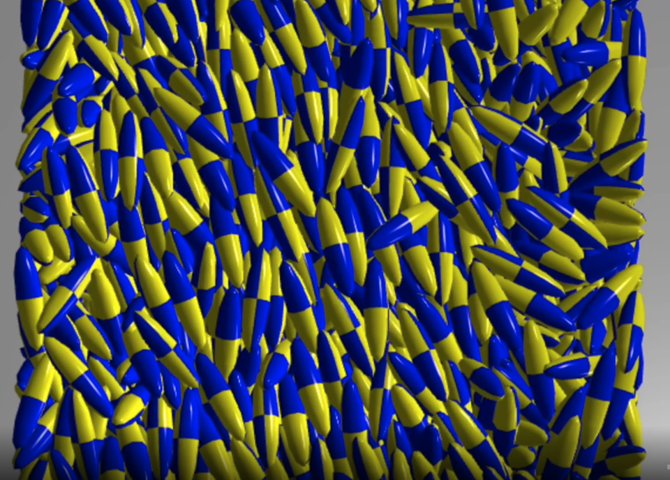
And in this simulation, as we know, due to the Jeffery rotation, the non-spherical grains arrange themselves in similar orientations. An example of this is shown in the following figure:

This can be described using the distribution of angles in which the particles can be found in any given moment. This angle is measured towards the long side of the grain from the direction vector of the flow (so its in the figure of Uniplanar Jeffery motion).

Algorithm

The shown algorithm is written in Python. First we need a function to filter out the shear zone. For this, we just take method shown in Approximating the shear zone in split bottom granular material simulations using simple function fitting and put it into a single function:

def filter_shear_zone_with_fitting(coords, vs):
    def vel_estimator_func(coord, transition_rate, y_displacement, x_lin, x_quad, z_lin, z_quad):
        x = coord[0]
        y = coord[1]
        z = coord[2]
        return np.tanh(y_displacement + (y + x*x_lin + x*x*x_quad + z*z_lin + z*z*z_quad)*transition_rate)

    def vel_estimator_func_derivative_y(coord, transition_rate, y_displacement, x_lin, x_quad, z_lin, z_quad):
        return transition_rate * (1 - vel_estimator_func(coord, transition_rate, y_displacement, x_lin, x_quad, z_lin, z_quad)**2)

    fitParams, fitCovariances = optimize.curve_fit(
        vel_estimator_func, [coords[:, 0], coords[:, 1], coords[:, 2]], vs[:, 0])

    gradient_from_fit = - \
        vel_estimator_func_derivative_y(
            [coords[:, 0], coords[:, 1], coords[:, 2]], *fitParams)

    zone_filter = gradient_from_fit < -1.3

    return zone_filter

Where we again used 1.3 as the threshold for filtering the shear zone, this can change though on a per-simulation basis.

Now this must be executed for all available output files of a run, with the same particles, so we need to open all files in the directory of the simulation, then execute the steps for each file and aggregate the results:

import numpy as np
import vtkmodules.all as vtk
from vtkmodules.util.numpy_support import vtk_to_numpy
import re

# This is the folder that we used in this example
foldername = "0.184202_0.184202_0.0736806"
files = os.listdir(f"../outfiles/{foldername}/")
[a, b, c] = list(map(float, foldername.split('_')))
# If the grain is flat or not
## If it is flat, then we will need to use the sides for measuring the angle
is_z_longest = np.argmax([a, b, c]) == 2

all_shear_angles = np.array([], dtype=np.float64)

for file in files:
    # Filter out those output files that contain the particle angles and positions
    res = re.search(r"dump\d+\.superq\.vtk", file)
    if not res:
        continue
    print(file)
    filename = file

    # Open file with vtk reader
    reader = vtk.vtkPolyDataReader()
    reader.SetFileName(f"../outfiles/{foldername}/{filename}")
    reader.Update()
    output = reader.GetOutput()

    # Load data: coordinates, velocities, orientations
    coords = vtk_to_numpy(output.GetPoints().GetData())
    vs = vtk_to_numpy(output.GetPointData().GetArray(3))
    orientations = vtk_to_numpy(output.GetPointData().GetArray(8))

    # Filter out the shear zone
    zone_filter = filter_shear_zone_with_averaging_on_grid(coords, vs)
    filtered_orientations = orientations[zone_filter]

    # Tis contains the (0,0,1) vector in the local coordinate system of each grain, which is then converted to the global coordinate system this easily
    filtered_vectors = filtered_orientations[:, [2, 5, 8]]

    # It the particle is flat, we rotate this vector by 90°
    if not is_z_longest:
        tmp_vals = np.copy(filtered_vectors[:, 0])
        filtered_vectors[:, 0] = -filtered_vectors[:, 1]
        filtered_vectors[:, 1] = tmp_vals
    # Flip vectors that point backwards, since we only measure between [-90° <-> 90°]
    filtered_vectors[filtered_vectors[:, 0] < 0] *= -1

    # Transform the vectors into angles
    filtered_angles = np.arctan2(
        filtered_vectors[:, 1], filtered_vectors[:, 0])

    # Append the angles
    all_shear_angles = np.append(all_shear_angles, filtered_angles)

Where files is an array containing the filenames of all the output files of the run.

Then we can just make a histogram out of all_shear_angles:

import plotly.express as px

# Number of bins in histogram
bin_count = 100
hist, bin_edges = np.histogram(
    all_shear_angles*(180 / np.pi), bins=bin_count, density=True)
bin_midpoints = (bin_edges[:-1] + bin_edges[1:]) / 2

fig = px.bar(x=bin_midpoints, y=hist, labels=['Angle distribution'], )
fig.update_layout(barmode='group', bargap=0.0, bargroupgap=0.0,
                  xaxis_title="Angle [°]", yaxis_title="Probability")
fig.show()

Which results in the following figure:

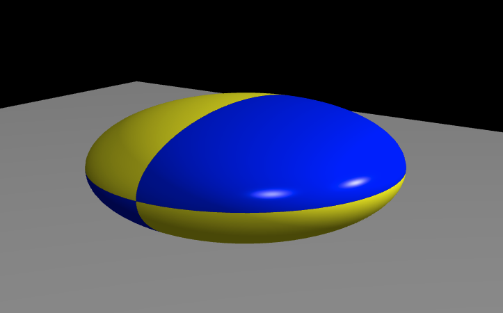
Remember, this example was done for the ellipsoidal particle of the following parameters:

Which is flat actually and looks like this: